Math Formulas within Posts
(Warning: this post was written when Wordpress was used to generate the blog. Quicklatex is no longer used. MathJax remains the tool used for math rendering). This post gives a few recipes to integrate mathematical formulas in html pages. This site uses MathJax, a javascript implementation of Latex.
Introduction
InvestmentMath uses two Wordpress plugins to display formulas: MathJaxand QuickLaTex.
We’ll first introduce MathJax.
MathJax : Adding LaTex formulas within posts
MathJax is an open-source (everyone can edit or read the source code) rendering engine for math formulas written in \(LaTeX\). It uses Javascript, so the rendering is done on the client-side. It preserves the server resources; however, slow clients will have significant loading times. According to its website, it uses plain ol’ CSS and web fonts, which means that its rendering is extremely clean and that it’s scalable. In addition, people with vision disabilities can zoom up to 400% using the MathJax menu which is obtained by right-clicking on any formula.
MathJax is amazingly powerful, and what’s more, the developers claim compatibility with all modern browsers. You can use it as a plugin with Drupal, Joomla!, MediaWiki, Wordpress and much more … It’s also used within the Ipython notebooks, a subject we will address in another post.
Now, here is an example showcasing the power of MathJax. Behold !
\[\log(P_{N})-\log(P_{0})=\sum_{k=0}^{K^{\delta}-1} \log(P_{t^{\delta}_{k+1}})-\log(P_{t^{\delta}_{k}})= \sum_{k=0}^{K^{\delta}-1} \log(P_{t^{\delta}_{k+1}}/P_{t^{\delta}_{k}})\]
You can right-click on this formula to discover the flexibility of MathJax and, in particular, to access the following code:
$$\log(P_{N})-\log(P_{0})=\sum_{k=0}^{K^{\delta}-1} \log(P_{t^{\delta}_{k+1}})-\log(P_{t^{\delta}_{k}})= \sum_{k=0}^{K^{\delta}-1} \log(P_{t^{\delta}_{k+1}}/P_{t^{\delta}_{k}})$$
QuickLaTex: inserting LaTex graphics made with TikZ
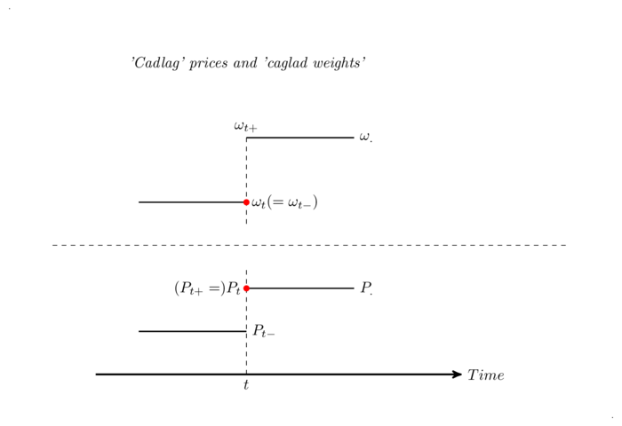
As you might have seen, some posts here use graphics generated in \(\LaTeX\) with TikZ. But, sadly, MathJax doesn’t support TikZ. We use QuickLaTex for that purpose. QuickLatex generates an image, which is then inserted in the web page. It also takes plain \(\LaTeX\) code like MathJax, but we only use it for its abilty to render TikZ graphics. It is nowhere near as powerful as MathJax. Let’s try an example, the very neat diagram from the Portfolio Returns post :
Here is the code :
[latex]
\begin{tikzpicture}[
    scale=5,
    axis/.style={very thick, ->, >=stealth'},
    important line/.style={thick},
    dashed line/.style={dashed, thin},
    pile/.style={thick, ->, >=stealth', shorten <=2pt, shorten
    >=2pt},
    every node/.style={color=black}
    ]
% Include tikz into local preamble
[+preamble]
     \usepackage{tikz}
     \usetikzlibrary{arrows}
[/preamble]
    \node at (-0.6,1.1) [] {\tiny .};
    \node at (2.2,-0.8) [] {\tiny .};
    \node at (.5,.9) [below] {\em 'Cadlag' prices and 'caglad weights' };
    \draw[axis] (-0.2,-.6)  -- (1.5,-.6) node(xline)[right]
        {$Time$}
    \draw[dashed line] (-0.4,0)  -- (2,0);
    \draw[important line] (0,0.2) -- (.5,.2) coordinate (A);
    \draw[important line] (.5,.5) coordinate (B) -- (1.0,.5) node[right, text width=1em] {$\omega_{.}$};
    \draw[dashed line] (.5,.1)  -- (.5,.5);
    \draw[dashed line] (.5,-.6)  coordinate (C) -- (.5,-.1);
     \fill[red] (A) circle (.4pt) node[right] {$\omega_{t}(=\omega_{t-})$};
     \node at (B)  [above] {$\omega_{t+}$};
     \node at (C) [below] {$t$};
     \draw[important line] (0,-.4) -- (.5,.-.4) coordinate (D) ;
     \draw[important line] (.5,-.2) coordinate (E) -- (1.0,-.2) node[right, text width=1em] {$P_{.}$};
     \fill[red] (E) circle (.4pt) node[left] {$(P_{t+}=)P_{t}$};
     \node at (D)  [right] {$P_{t-}$};
\end{tikzpicture}
[/latex]
Tikz code might look complicated but actually is not. It takes about an hour for a \(\LaTeX\) user to understand the logic. In addition, Tikz code can be directly generated through Geogebra and its friendly GUI!