Martingales
This post introduces the notion of a martingale. The concept is key to finance, but it is also central in stochastic analysis. A martingale is a process which, at any given date, is expected to remain at its current level in the future. In other words, its future increments (called martingale differences) are expected to be equal to zero. Picking a variable \(X_{T}\), the process \((E_{t}[X_{T}])_{t \in [0,T]}\) is a martingale which is ‘closed’ by \(X_{T}\). The concept is illustrated using the discretized version of a martingale, namely a random walk with centered increments.Continuous time martingales with (loosely speaking) independent identically distributed increments are called Levy martingales. The post introduces two Levy martingales, the Brownian motion and the compensated Poisson proces.
The definition
The concept of a martingale is probably the most important concept in mathematical finance. A martingale is a stochastic process which is expected at any point in time to remain at the same level in the future.
To formally introduce the definition, we need to set up the landscape. We need a probability space \((\Omega,{\cal F},P)\) where \(\Omega\) is the sample space, \({\cal F}\) is a sigma-algebra and \(P\) is a probability measure on \((\Omega,{\cal F})\). The sigma algebra is decomposed into a filtration1. \(({\cal F}_{t})_{t \in \mathbb{T}}\), i.e. an increasing family of sigma algebras. The index set \(\mathbb{T}\) can for instance be the set of natural numbers \(\mathbb{N}\) or the positive real line \([0,\infty[\). The filtration models the flow of information. Conditional expectations with respect to an element of the filtration, \(E[\cdot|{\cal F}_{t}]\) will be noted \(E_{t}[\cdot]\).
In this context, a martingale is a stochastic process \((M_{t})_{t \in \mathbb{T}}\) adapted to the filtration (i.e. for each \(t\), \(M_{t}\) is \({\cal F}_{t}\) measurable) such that:
\[M_{t_{0}}=E_{t_{0}}[M_{t_{1}}],\, \forall t_{1} \geq t_{0}.\]
A martingale can be obtained by first choosing a (\({\cal F}\)) random variable \(\xi\) and setting:
\[M_{t}=E_{t}[\xi].\]
The random variable \(\xi\) is said to close the martingale.
Martingale differences
When \(\mathbb{T}=\mathbb{N}\), we can look at the martingale difference \(\Delta M_{t}=M_{t}-M_{t-1}\). We have:
\[E_{t}[\Delta M_{t+k}]=0,\, k \geq 1,\]
i.e. the martingale difference is conditionally (and hence unconditionally) centered. We also have (using the tower law of conditional expectations):
\[E_{t}[\Delta M_{t+h}\Delta M_{t+k}]=0,\, \forall h,k \geq 1,\,h\neq k.\]
Martingale differences have zero conditional (and thus unconditional) covariance. The martingale difference process \((\Delta M_{t})_{t \geq 1, t \in \mathbb{T}}\) is a sequence of uncorrelated random variables. The variables need not be independent.
Simulating discrete time martingales
In practice, a simple way to simulate a discrete time martingale consists in drawing \(I\) sets of independent increments \((\Delta m^{i}_{t})_{t \geq 1, t \in \mathbb{T}, 1 \leq i \leq I}\) from a given distribution using a pseudo random numbers generator. One can then compute the martingale by cumulating the random draws:
\[m_{0}=0,\] \[m^{i}_{t}=\sum_{k=1}^{t}\Delta m^{i}_{k}.\]
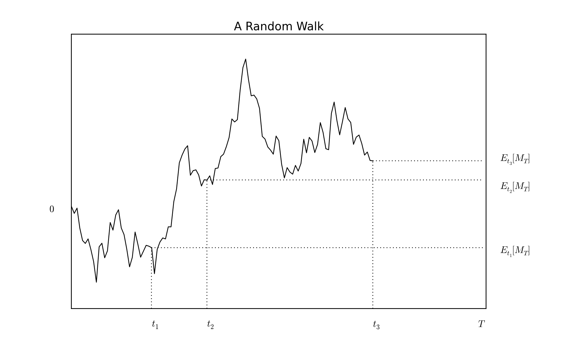
The index \(i\) plays the role of \(\omega\) (the ‘event’), it indexes the drawn trajectory. The following graph shows a particular outcome (a particular sample), where increments are drawn from the standardized Gaussian law. The graph illustrates the key property of martingales for three chosen dates. As of each date, the expected value of the martingale is represented by a horizontal dashed line. In this example, the index set is an interval \([0,T]\) and the martingale is closed by \(M_{T}\).
Two interpretations
Several interpretations illustrate the importance of martingales for finance.
A martingale can be seen as the cumulated pay-off of a player engaged in a sequence of games where each game has a zero expected pay-off (fair game).
Financial instruments promise pay-offs such coupon payments or dividends. Any such payment can be thought of as the closing random variable of a martingale which is simply the expected value of the payment. The expected value of the payment fluctuates as investors acquire information on it.
We will put a lot of emphasis on this latter perspective when discussing stochastic integrals.
Expected pay-offs are necessarily a key ingredient in the pricing of financial instruments.
From random walks to Levy martingales
We have seen how a discrete time martingale could be simulated, drawing independently from a single distribution. The result is called a random walk2. Discrete time modeling is very efficient as it allows to avoid thorny technical questions. However, discretization relies on sampling assumptions which can sound quite arbitrary. One can therefore wish to think of a discrete time process as resulting from sampling an underlying continuous time process. This opens up a number of interesting modeling issues. Here is an illustration.
If, starting from the previous random walk, one refines the initial grid adding midpoints in between each set of successive dates, the original increments can be additively decomposed into two pieces:
\[\Delta M_{t}=M_{t}-M_{t-1}=(M_{t}-M_{t-1/2})+(M_{t-1/2}-M_{t-1}).\]
One can divide intervals in three, four or \(n\) subsets of equal length. Imposing that the subdivivisions always entail independent, identically distributed (i.i.d.) and centered increments preserves the structure applied to the initial random walk martingale. When the operation can be carried out for any natural number \(n\), we say that the initial distribution is infinitely divisible.
Levy processes are designed on this idea3. The marginal law of any term \(M_{t}\) is infinitely divisible. The main examples of infinitely divisible distributions are Gaussian, Poisson and compound Poisson distributions. Using these, we get the Brownian process, the Poisson process or the compound Poisson process. In our case, the increments have to be centered to obtain a martingale. This is achieved by removing an adequate drift from the original process if needed, a procedure called ‘compensation4’ (thus the term ‘Compensated Poisson process’).
The Brownian process has continuous sample paths whereas processes of the Poisson type are cadlag (continuous on the right, with limits on the left) but have jumps. Paraphrasing this in the context of our interpretation of martingales as expectation of future dated outcome \(\xi_{T}\), we can say that in the case of a Brownian martingale, information acquisition is rather evenly spread over time while in the compensated Poisson case, information comes in a lumpy way, the timing of the news being random.
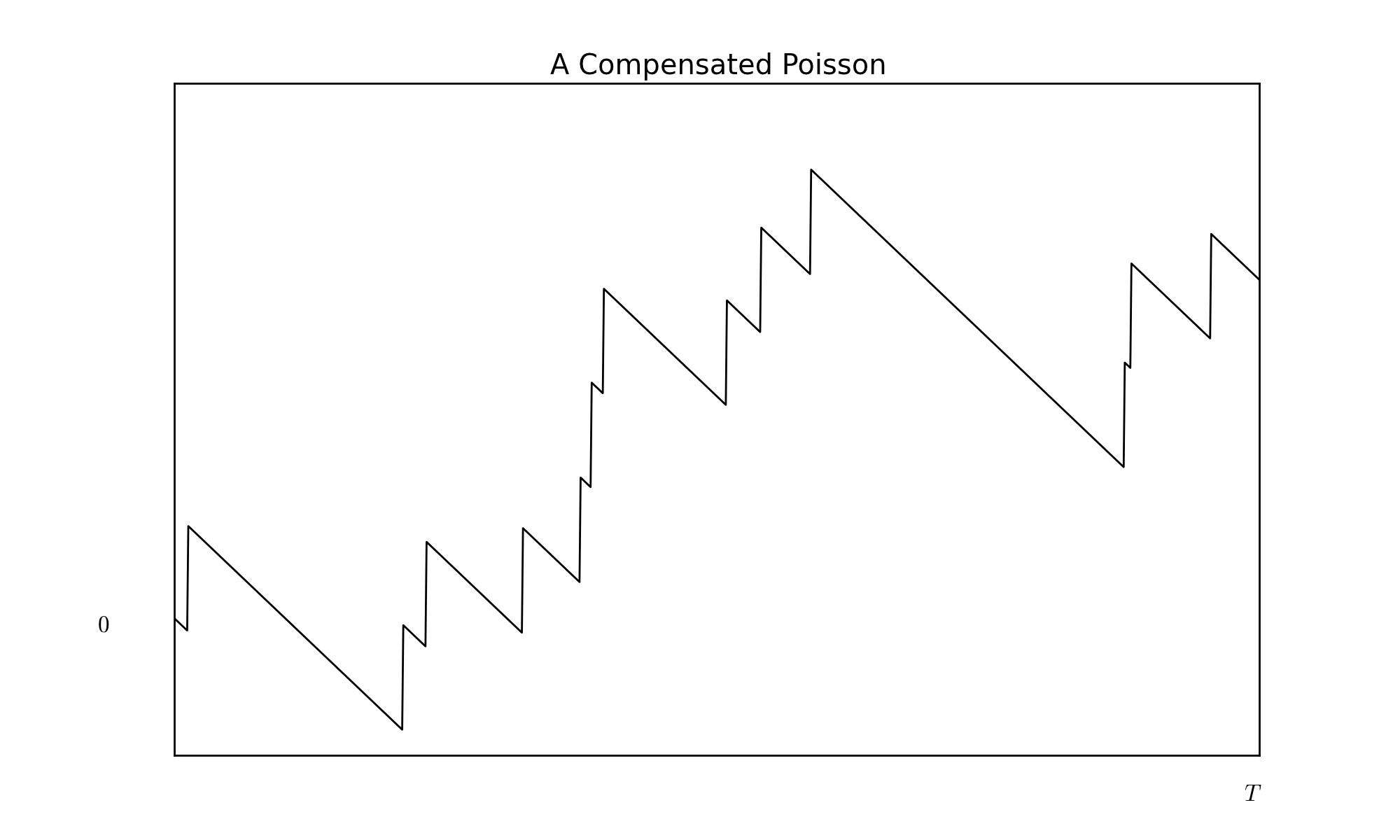
To illustrate the diversity of martingale trajectories, I simulate below a compensated Poisson process. This is done in the following way. We independently draw \(I\) sets of \(N\) random (‘inter-arrival’) times using the exponential distribution of parameter (intensity) \(\lambda\). This gives us a set of dates \((t^{i}_{k})_{1\leq k \leq N, 1 \leq i \leq I}\). We then define: \[m^{i}_{t}=\max \{
j | \sum_{k=1}^{j}t^{i}_{k} \leq t \}-\lambda t,\, t \leq
\sum_{k=1}^{N}t^{i}_{k}.\] This is an example of a (compensated) point process5. Here is a graph of a particular trajectory (drawn using \(\lambda=1\)).
Keep in mind that although it might not be obvious from the trajectories, the compensated poisson process has independent increments. As seen from the graph, the compensated Poisson process falls at a rate \(\lambda\) except at jump dates. Changing the jump size from \(1\) to \(-1\) (which is equivalent to applying a symmetry around \(0\) on the \(y\) axis) would create a process that rises at a steady rate \(\lambda\) except at jump dates where it falls. The increments of such a process have negative skewness (a lot of small upward moves and a few big downward moves), which is an empirical feature of market prices. This is in contrast to the Brownian motion, which increments have a symmetric distribution.
In the above example, jumps have a fixed size. One could instead make jump size random, drawn independently from other variables as well as independently from one jump to another. The range of available Levy processes and their corresponding martingales is thus very large. The potential of Levy processes to model empirical features of financial data has triggered a lot of research over the past decade.
Finally, as an illustration of the power and elegance of the martingale perspective in stochastic analysis, I close this introduction with two important characterization results :
A process \((B_{t})_{t \in \mathbb{R}_{+}}\) with \(B_{0}=0\) and continuous trajectories is a Brownian motion if and only if \(B_{t}^{2}-t\) is a martingale (Levy’s characterization of the Brownian motion).
A point process \((P_{t})_{t \in \mathbb{R}_{+}}\) is a Poisson process of intensity \(\lambda\) if and only if \(P_{t}-\lambda t\) is a martingale (Watanabe’s characterization of the Poisson process).
Links
In continuous time, this filtration has to satisfy the so-called ‘usual conditions’, namely the filtration is assumed to be continuous on the right and complete - cf. for instance Protter, Stochastic Integration and Differential Equations, Springer.↩︎
A random walk need not have centered increments.↩︎
See for example D. Applebaum, Levy Processes and Stochastic Calculus, Cambridge Studies in Advanced Mathematics.↩︎
Any Levy process \((X_{t})\) such that \(E[|X_{t}|]<\infty\) can be ‘compensated’ and thus turned into a martingale.↩︎
A Poisson process is defined as above, but omitting the compensating term \(\lambda t\). Relaxing the exponential assumption on the distribution of the ‘inter-arrival’ times, we get a more general point process.↩︎


