Portfolio Returns
This post introduces the dynamics of the value of a portfolio. It starts with an unfrequently rebalanced portfolio: portfolio weights are assumed ‘simple’, i.e. piecewise constant. In this case, the portfolio value dynamics is trivial. More complex rebalancing schemes can be approximated using sequences of simple weighting schemes, just as a continuous function can be approximated using peacewise constant functions. The dynamics of portfolio value is then given by a stochastic integral. This example stresses an essential feature of stochastic integrals: portfolio weights (integrands) are forced to lag prices (integrators).
Portfolio returns in the absence of rebalancing
In previous posts, we have looked at the returns of a given security, which we have defined using its price as well as its income stream. Whenever we speak of a price, we imply that it is a value attached to a unit, and that several units can be bought or sold. Value decomposes into prices and quantities.
If \(n^{i}_{t}\) is the quantity of asset \(i\) with price \(P^{i}_{t}\), the corresponding value is simply \(V^{i}_{t}=n^{i}_{t}P^{i}_{t}\). A portfolio invested in assets \(i=0,\ldots,N\) with quantities \((n^{i}_{t})_{0\leq i \leq N}\) has an overall value of:
\[V_{t}=\sum_{i=0}^{N}n^{i}_{t}P^{i}_{t}.\]
If quantities are unchanged between two dates \(t_{1}\) and \(t_{2}\), value evolves as a result of price changes:
\[V_{t_{2}}-V_{t_{1}}=\sum_{i=0}^{N}n^{i}_{t_{1}}(P^{i}_{t_{2}}-P^{i}_{
t_{1}}),\]
and the return of the portfolio is (assuming values and prices are strictly positive):
\[\frac{V_{t_{2}}}{V_{t_{1}}}-1=\sum_{i=0}^{N}\frac{n^{i}_{t_{1}}P^{i}_{
t_{1}}}{V_{t_{1}}}\frac{P^{i}_{t_{2}}}{P^{i}_{t_{1}}}-1
=\sum_{i=0}^{N}\omega^{i}_{t_{1}}(\frac{P^{i}_{t_{2}}}{P^{i}_{t_{1}}}-1)
.\]
where:
\[\omega^{i}_{t_{1}}=\frac{n^{i}_{t_{1}}P^{i}_{t_{1}}}{V_{t_{1}}}=\frac{ V^{i}_{t_{1}}}{V_{t_{1}}},\]
is the share of portfolio value which is invested in asset \(i\) at date \(t_{1}\). The shares by definition sum to \(1\):
\[ \sum_{i=0}^{N}\omega^{i}_{t_{1}}=1.\]
In between such dates, portfolio returns are thus linear in the returns of the underlying assets. They do not look linear in the log returns.
Rebalancing
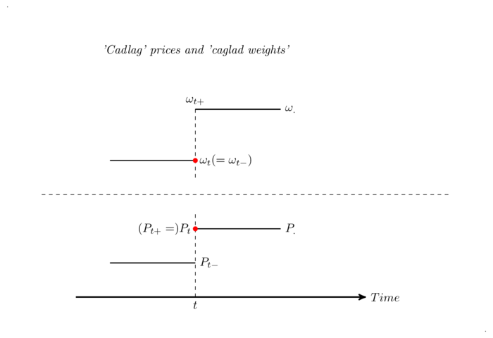
A rebalancing date \(t\) is a date when a decision is made to modify portfolio composition. Portfolio composition is changed from the inherited one \((\omega^{i}_{t})_{0 \leq i \leq N}\) to a new one \((\omega^{i}_{t_{+}})_{0 \leq i \leq N}\). Once the decision to rebalance is taken, implementation takes an arbitrarily small amount of time, leading to the assumption that at \(t\), the old portfolio composition prevails while the new one prevails right after \(t\), at \(t+\) (i.e. at any time \(t+\epsilon, \epsilon\>0\), \(\epsilon\) sufficiently small).
If there are no frictions in the trading process, portfolio value is preserved by rebalancing:
\[V_{t}=V_{t_{+}}.\] I thus assume here that portfolio weights are piecewise constant, continuous on the left and with limits on the right (caglad, ‘continue à gauche avec limites à droite’). This does not play a role when price processes are continuous (when prices follow standard diffusion processes for instance), but it does when price processes may jump, in which case the crucial question is whether portfolio weights are allowed to jump in sync with the price processes. Concretely, if the price process jumps, as a Poisson process does, from \(P^{i}_{t-}\) to \(P^{i}_{t}\), can the portfolio policy knowingly benefit from that jump? The usual theory rules this out: price processes are cadlag (‘continue à droite avec limites à gauche’) and portfolio weights are caglad; the jump is observed at \(t\), when the rebalancing decision is taken; portfolio weights lag price jumps1. The profit accruing from the price jump at a rebalancing date \(t_{k}\) is a function of the portfolio decision at the last rebalancing date \(t_{k-1}\):
\[n^{i}_{t_{k-1}+}(P^{i}_{t_{k}}-P^{i}_{t_{k-}}).\] Concretely, as explained above, placing a trade in markets takes a little bit of time, whichever technology is used. Therefore, the information set on which a decision is made predates the information set at trading time. The restriction is thus quite natural.
Portfolio dynamics
Given assets and their price processes as well as a set \((t_{k})_{0 \leq k \leq K}\) of rebalancing dates with holding policies \((n^{i}_{t_{k}})_{0 \leq i \leq N}\), we can now trivially compute the dynamics of portfolio value:
\[V_{t_{K}}-V_{t_{0}}=\sum_{i=0}^{N}\sum_{k=0}^{K-1}n^{i}_{t_{k}+}(P^{i}
_{t_{k+1}}-P^{i}_{t_{k}}).\]
This is valid in the absence of trading costs. The inside sum in this formula can be taken as the definition of an integral for simple portfolio quantities (piecewise constant caglad). This is precisely the starting point of the definition of stochastic integrals (see for example Protter, Stochastic Integration and Differential Equations). We can thus write:
\[V_{t_{K}}-V_{t_{0}}=\sum_{i=0}^{N}\int_{t_{0}}^{t_{K}}n^{i}_{t}dP^{i}\_
{t},\]
or:
\[dV_{t}=\sum_{i=0}^{N}n^{i}_{t}dP^{i}_{t},\]
\[\frac{dV_{t}}{V_{t}}=\sum_{i=0}^{N}\omega^{i}_{t}\frac{dP^{i}_{t}}{P^{ i}_{t}}.\]
Portfolio value thus follows a stochastic differential equation2, and even a geometric one when prices are strictly positive. It is the purpose of integration theory to demonstrate that integration can be extended to more complex trading policies than the piecewise constant ones described above, and in particular to policies of continuous rebalancing. We will allow fairly general trading rules in these notes.
An important practical observation is that in continuous time, geometric returns and log returns are linearly related:
\[d\log(P_{t})=\frac{dP_{t}}{P_{t}}-\frac{1}{2}\frac{d[P]_{t}}{P_{t}}.\]
The portfolio log return is thus a linear combination of the log returns of the assets. This is quite neat since it allows to build log-normal models, i.e models where both prices and portfolio value follow log-normal models…
PS: Computing portfolio returns thus naturally leads us to using stochastic integrals. A more mathematical glimpse into the definition of stochastic integrals will be provided in another post. In particular, the fact that stochastic integrals preserve the martingale property is key to the subject of this blog.