Math for Index Construction: Introduction
This series of posts discusses methods relevant for equity index construction. Although portfolio construction typically subsumes index construction, there is a specific flavour to index construction: index rules need to be relatively simple and transparent. They are fully disclosed by index providers and implemented in a mechanical way. This narrows the possibilities. Posts in this series will therefore concentrate on simple and transparent rules to build equity portfolios. It will cover some existing constructions as well as new ones, with special attention brought to the conceptualization behind each approach.
Indices and their Parametrizations
I start by describing securities and prices, so as to be able to define the market index and set the scene for more complex constructions.
I suppose we have \(N\) stocks, which distribute no dividends. A useful innocuous convention is to assume that there are exactly \(1\) unit of stocks available in the market, and that any real number \(\Delta n\) of that stock can be traded. One can always apply fictitious split or reverse split to map real data to that convention. The vector of stock prices is \((p_i)_{1\le i \le N}\). As a result, outstanding market value is just: \[\sum_{i=1}^N p_i.\] I will assume all prices are strictly positive and as a simplification, all positions are strictly positive as well, i.e. portfolios are long-only.
An index is a self-financed portfolio which value has been arbitrarily set to some amount, say \(1\)$, at a specific date. These choices are arbitrary and irrelevant insofar as our attention is on the index as a portfolio policy prescription which can be scaled in a straightforward way at any level of wealth. The policy is applied by splitting wealth \(W_t\) at date \(t\) using the portfolio weights of the index, \((\omega_{i,t})_{1\le i\le N}\). Equivalently, the policy is applied by scaling the numbers of shares of the index \((n_{i,t})_{1\le i\le N}\) by a factor \(\lambda_t\) such that: \[\lambda_t \sum_{i=1}^N n_{i,t} p_{i,t}=W_t,\] and holding the scaled numbers of shares \((\lambda_t n_{i,t})_{1\le i\le N}\). One can easily see that the rebasing of the index to another date and /or initial level doesn’t change the policy prescription. As a result, we can describe an index as a sequence of portfolio weights (indexed by time) or by a sequence of numbers of shares.
Behind a vector of weights there are \(N-1\) degrees of freedom (portfolio weights belong to the simplex - see below), whereas a vector of numbers of shares has \(N\) degrees of freedom. Each vector \(n_t\) can actually be specified up to any strictly positive factor since the portfolio rule will entail adapting it to the wealth of the portfolio under consideration. All that matters thus is numbers of shares up to a homothecy, and this entails \(N-1\) degrees of freedom as well. I call numbers of shares up to a common scale pseudo-numbers of shares, and note them \([m_t]\). Pseudo-numbers of shares belong to the projective positive orthant which I will describe below. They can be thought as the set of ratios \((n_i/n_1)_{2 \le i \le N}\) (provided \(n_1\) is not zero). Expressing the number of shares at each date for a wealth level of \(1\)$, we get the representative \((\omega_i/p_i)_{1\le i\le N}\). The other way round, for \(m\in [m]\), the portfolio weights can be recovered through: \[\omega_i=\frac{m_i p_i}{\sum_{j=1}^{N}m_j p_j},\, 1\le i \le N,\] and we see that this formula gives the same portfolio weights prescription for all \(m\in [m]\). Finally, fixed pseudo-numbers of shares correspond to buy-and-hold indices.
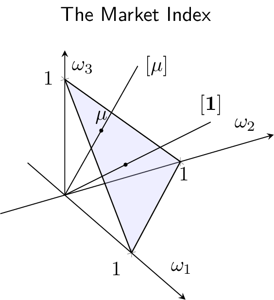
In the above setup, the portfolio weights of the maket index are: \[\mu_i=\frac{p_i}{\sum_{i=1}^N p_j},\, 1\le i \le N,\] i.e. the market cap weights which belong to the probability simplex. Obvioulsy, the portfolio weights drift with stock prices. Things are simpler when looking at pseudo-numbers of shares as numbers of shares are constant: the portfolio rule is buy-and-hold and the corresponding pseudo-numbers of shares are \(\mathbf{1}_N\) up to a homothecy, a construct that I will note \([\mathbf{1}_N]\) or simply \([\mathbf{1}]\) (the dimension is then implicit).
One should distinguish the market index from the market portfolio. The market portfolio is the portfolio which holds all outstanding shares. Of course, it follows the strategy embedded in the market index.
An important observation is that using market cap weights in a portfolio return calculation is equivalent to taking the market portfolio as the numeraire, i.e. all prices and returns are measured as a fraction of market value. Accordingly, the relationship: \[\sum_{i=1}^N \mu_i=1,\] just says that the value of the market portfolio is constant when the market portfolio is used as the numeraire.
Finally, using the market portfolio as the numeraire, the relationship between portfolio weights and pseudo-numbers of shares can also be written as: \[\forall m \in [m],\, \omega_i=\frac{m_i \mu_i}{\sum_{j=1}^{N}m_j \mu_j},\, 1\le i \le N,\] \[[m]=[(\omega_i/\mu_i)_{1\le i\le N}].\]
Geometric Constructions in the Positive Orthant
From the above discussion, we see that two mathematical constructions in the positive orthant \(\mathbb{R}^N_+\) are handy to track portfolios and indices. The most common tool is the simplex \(\Delta_N\) of long-only portfolio weights: \[\Delta_N=\{\omega=(\omega_i)_{1\le i\le N}| \omega_i \ge 0,\, 1\le i\le N, \sum_{i=1}^{N} \omega_i=1\}.\] A less common construction is the space of rays which is the space of equivalent classes obtained by identifying the vectors \(x\) and \(y\) whenever there is a strictly positive scalar \(\lambda\) such \(x=\lambda y\) i.e.: \[x\sim y \iff \exists \lambda>0,\, x=\lambda y,\] \[{\cal P}^N_+=\mathbb{R}^N_+/\sim.\] This is the set of half-lines in the orthant that are anchored at the origin. In our vocabulary, \({\cal P}^N_+\) is the set of pseudo-numbers of shares and I note \([x]\) the ray that goes through \(x\). We’ll explore \({\cal P}^N_+\) in more details in the next post.
Illustrations
I illustrate these constructions in the case of the market index below in Figure \(1\) assuming there are three stocks. The vector of portfolio weights of the market index is \(\mu\), which belongs to \(\Delta_N\). The pseudo-numbers of shares of the market index is the ray \([\mathbf{1}_N]\) i.e. the ray that goes through \(\mathbf{1}_N\). Although over time \(\mu\) will move as in the animation below (Figure \(3\)), the pseudo-numbers of shares vector is fixed.
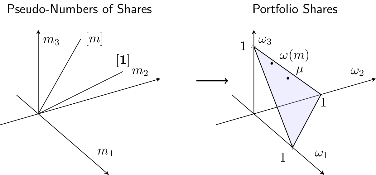
In the following graph, I illustrate how one goes from indices specified through pseudo-numbers of shares (here, the market index \([\mathbf{1}_N]\) and an arbitrary portfolio \([m]\)) to the representation of the same portfolios in the portfolio weights space (\(\mu\) for the market index and \(\omega\) for the other index) using the formulas at the end of the previous section for a given set of prices encoded in \(\mu\).
The Market Index: Practical Considerations
The description of the market index above is very stylized. First, most equity indices select a subset of listed stocks, and adapt it over time. The investment universe is therefore not fixed. A market capitalization threshold is usually selected. As a result, over time, some stocks fall below the threshold and get replaced by stocks that have moved above the threshold. This is usually refered to as insertions and deletions. The oustanding number of shares of a stock is also typically not fixed. There are so-called ‘corporate actions’ such as capital issuance, share repurchases, mergers… Finally, stocks distribute dividends which indices need to reinvest. Despite these frictions, the above simplified framework is a good approximation to reality. The index turnover of market indices is typically very low.
Alternatives to Market Indices
The following blog posts will deal with alternative index constructions. Non market-cap indices are very common. They integrate non-price related information on securities and reflect that information in positions. We will assume the additional information comes as a vector of stock characteristics which we will call the score. We will concentrate on methods to integrate that information, along with market capitalization shares, to form an index. The particular interpretation of the score might vary from one application to another. The additional characteristic can be the ratio of a fundamental metric to the price, i.e. a valuation ratio. This is the setup that leads to so-called value indices, which are the main (but not exclusive) focus in what follows.