Index Construction in the Space of Rays

December 2nd, 2025

In this post, I start looking at a multiplicative method. Multiplicative methods are best understood by working with pseudo-numbers of shares in the projective orthant. The market pseudo-numbers of shares are perturbed in proportion to a score built from stock characteristics. The market shares are shifted proportionately and then radially projected on the simplex. I detail the case where the stock characteristic is a valuation ratio, where the method has a natural interpretation. Numerous important practical indices arise from this setup such as the equal-weight index, the diversity-weighted index and fundamental ones. Value indices based on the multiplicative method generalize the fundamental-index construction.

Aitchinson Geometry in the Projective Orthant

The following construction is usually called Aitchinson’s geometry by statisticians, and is used in statistical analysis of compositional data. A good mathematical reference is Faugeras[2024].

The space of rays (half-lines anchored at the origin) in the positive orthant can be endowed with a vector space structure, i.e. an operation of addition on rays which gives it a group structure, and a scalar action of reals on rays. I will write below \(m\) to denote an arbitrary point in \([m]\).

I will use the following notation:

Addition of rays: \([m]\oplus [p]=[(m_i p_i)_{1\le i\le N}]\),
Action of reals: \(\alpha \otimes [m]=[(m_i^\alpha)_{1\le i\le N}]\).

One can check that the neutral element for addition is \([\mathbf{1}_N]\) (\([\mathbf{1}_N]\oplus [m]=[m]\)). The operations satisfy the additional relationships required for a vector space:

\(1\otimes[m]=[m]\),
\(\alpha \otimes ([m]+[p])=\alpha \otimes [m]+\alpha \otimes[p]\),
\((\alpha+\beta) \otimes [m]=\alpha\otimes [m]+\beta\otimes [m]\),
\((\alpha\beta) \otimes [m]=\alpha(\beta \otimes [m])\).

Here are some observations to become more familiar with this setup:

the opposite of a ray \([m]\) is \(-1\otimes [m]=[(1/m_i)_{1\le i\le N}]\),
I note \([\omega]+(-1\otimes [p])=[\omega]\ominus [p]\),
\(\lambda\otimes[\mathbf{1}_N]=[\mathbf{1}_N]\),
given two rays \([m]\) and \([p]\) , we can combine them through \((1-\lambda)\otimes [m]\oplus \lambda \otimes [p]\), either to form a convex combination or to describe the line going through both points,
as a result, \((1-\lambda)\otimes [m]\oplus \lambda \otimes [p]=[m]\oplus \lambda \otimes [p]=\lambda \otimes [p].\)

Finally, we can endow \({\cal P}^N_+\) with a metric, called the Hilbert metric: \[d_H([m],[p])=\log\left(\frac{\max_{1\le i\le N}m_i/p_i}{\min_{1\le i\le N}m_i/p_i}\right),\] which is invariant to the choice of representatives in \([m]\) and \([p]\).

Remark (Exponential coordinates): We saw in the previous post that in exponential coordinates, the space of rays becomes the set of lines in \(\mathbb{R}^N\) that are parallel to the diagonal. Writing \(\theta=(\theta_i)_{1\le i\le N}\in \mathbb{R}^N\), these lines are: \[\theta+\gamma \mathbf{1}_N,\, \gamma \in \mathbb{R}.\] The vector space structure on \({\cal P}^N_+\) corresponds to the vector space structure induced on the space of such lines by the usual vector space structure of \(\mathbb{R}^N\) (quotient vector space).

\(\square\)

Perturbing the Market Index

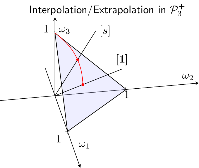
We consider a score \(s\) with strictly positive components, with its corresponding ray \([s]\). We wish to perturb the market index \([\mathbf{1}_N]\) using the tools just developed. To this end, we can consider the ray: \[[m]_{\lambda,s}=(1-\lambda)\otimes [\mathbf{1}_N]\oplus \lambda \otimes [s]=\lambda \otimes [s]=[(s_i^\lambda)_{1\le i\le N}],\] for \(\lambda \ge 0.\) We have: \[d_H([m]_{\lambda,s},[\mathbf{1}_N])=\log\left(\frac{\max_{1\le i\le N}s_i^\lambda}{\min_{1\le i\le N}s_i^\lambda}\right).\] The distance between the market index and the new index is zero for \(\lambda=0\), and grows with \(\lambda\). The situation is materialized on Figure \(1\) below.

From a practical standpoint, it is important to know which stocks get overweight and which are underweight against the market index. We have: \[[\omega]_{\lambda,s}=[(m_i\mu_i)_{1\le i\le N}]=[\mu] \oplus [m]_{\lambda,s}=[\mu] \oplus(\lambda \otimes [s]),\] or: \[[\omega]_{\lambda,s}\ominus [\mu]=\lambda \otimes [s],\] and since \(\omega_{\lambda,s}\) belongs to the simplex: \[\omega_{\lambda,s,i}=\frac{s_i^\lambda \mu_i}{\sum_{j=1}^{N} s_j^\lambda \mu_j}.\] We can pick as representative of \([s]\) the vector \(\tilde{s}\) with components such that: \[\sum_{j=1}^{N} \tilde{s}_j^\lambda \mu_j=1,\] and with that choice we get: \[\frac{\omega_{\lambda,s,i}}{\mu_i}=\tilde{s}^\lambda_i.\] As a result: \[\omega_{\lambda,s,i} \ge \mu_i \iff \tilde{s}^\lambda_i\ge 1.\]

A benefit of mapping the score \(s\) to the pseudo-numbers of shares \([m]\) is that it leads to a clear trading process driven by \([s]\). Indeed, the portfolio remains buy-and-hold as long as \([s]\) remains fixed¹.

The Case of Value Indices

Just as any strictly positive number \(y\) can be related to another strictly positive number \(x\) through \(y=x (y/x)\), any long-only portfolio with the same investment universe as the market index can be related to it using the multiplicative methods. The construction is useful though when the score has a natural interpretation, as in the case I detail now. In this example, the score is a valuation ratio \(e_i/p_i\) where \(e_i\) is the fundamental metric of stock \(i\). The ratio \(e_i/p_i-1\) is the percentage deviation between \(i\)’s stock price and its anchor. This deviation need not average to zero across stocks. I note \(\pi\) the intersection of \([e]\) with the simplex, just like \(\mu\) is the intersection of \([p]\) with the simplex.

Thus: \[s_i=\frac{e_i}{p_i},\, 1\le i\le N.\] A stock \(i\) is said to be relatively cheap if it has a high score and relatively expensive if it has a low score. The Hilbert distance \(d_H([s],[\mathbf{1}_N])=d_H([\pi]\ominus[\mu],[\mathbf{1}_N])\) between the score and the identity of \({\cal P}^N_+\) is called a value spread by practitioners, as it measures the valuation gap between the most expensive and the cheapest stock.

We have: \[[s]=[e]\ominus[p]=[\pi]\ominus[\mu],\] and: \[[m]_{\lambda,s}=\lambda \otimes ([\pi]\ominus[\mu])=[(\frac{\pi_i^\lambda}{\mu_i^\lambda})_{1\le i\le N}].\] As a consequence: \[[\omega]_{\lambda,s}=[(\mu_i m_i)_{1\le i\le N}]=[\mu]\oplus \lambda \otimes([\pi]\ominus [\mu]),\] or: \[[\omega]_{\lambda,s}\ominus [\mu]=\lambda \otimes([\pi]\ominus [\mu]).\] Since \(\omega\) lies in the simplex: \[\omega_{\lambda,s,i}=\frac{\left(\frac{\pi_i}{\mu_i}\right)^\lambda \mu_i}{\sum_{j=1}^{N} \left(\frac{\pi_j}{\mu_j}\right)^\lambda \mu_j},\, 1\le i\le N.\]

The portfolio shares have a very simple expression in the case \(\lambda=1\): \[\omega_{1,s}=\pi.\]

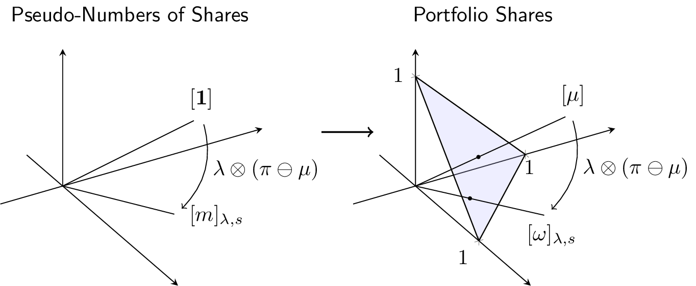
The overall construction is summarized in the graph below, stressing that both the market pseudo-numbers of shares and market shares are applied the same translation when viewed as rays: \[[m]_{\lambda,s}=[m]_{\lambda,s}\ominus[\mathbf{1}_N]=\lambda \otimes ([\pi]\ominus[\mu])=[\omega]_{\lambda,s}\ominus [\mu].\]

Key Examples

The equal weight portfolio is obtained by picking \([e]=[\mathbf{1}_N]\) and \(\lambda=1\). We indeed have \(e_i=e\) for all \(1\le i\le N\), and: \[\omega_i=\frac{\left(\frac{e}{\mu_i}\right) \mu_i}{\sum_{j=1}^{N} \left(\frac{e}{\mu_j}\right) \mu_j}=\frac{1}{N},\, 1\le i\le N,.\]

Relaxing the constraint \(\lambda=1\), we get the so-called diversity weighted indices: \[\omega_i=\frac{\mu_i^{1-\lambda}}{\sum_{j=1}^{N} \mu_j^{1-\lambda}},\, 1\le i\le N,.\]

As mentionned above, for \(\lambda=1\), the formula for a generic \(e\) leads to the fundamental index: \[\omega_i=\pi_i=\frac{e_i}{\sum_{j=1}^{N} e_j},\, 1\le i\le N,\] and choosing a different \(\lambda\) delivers the generalized fundamental indices: \[\omega_i=\frac{e_i^\lambda \mu_i^{1-\lambda}}{\sum_{j=1}^{N} e_j^\lambda \mu_j^{1-\lambda}},\, 1\le i\le N,\] which interpolates between the fundamental index and the market index.

Relative Performance of The Generalized Fundamental Indices

We will see in later posts that the relative performance of the above ‘value indices’ is tied to the relative dynamics of \(\pi\) and \(\mu\). In particular, we will see that for fixed \(\pi\), the ‘value indices’ beat the market when market cap shares move towards \(\pi\), and symmetrically, underperform when \(\mu\) moves away from \(\pi\). A generalized notion of distance will help make these statements rigorous. For fixed \(\pi\) again, these indices benefit from cycles in prices (they are noise harvesting). The dynamics of \(\pi\) has the power to derail these properties though. If \(\pi\) is smooth enough and does not chase prices, the fixed \(\pi\) intuition remains valid. As far as relative performance is concerned, generalized fundamental indices are noise-harvesting indices which bet that the underlying metrics \(e_i\) are smooth anchors for relative prices. In applied constructions, some care is needed to avoid having anchors that run after prices.

References

Faugeras[2024]: Faugeras O., An Invitation to Intrinsic Compositional Data Analysis Using Projective Geometry and Hilbert’s Metric, Working Paper, Toulouse School of Economics.

InvestmentMath