The Martingale Method in Continuous Time
This post describes the martingale method in continuous time. It should be read after this one. It illustrates the method on a simple example within the Black and Scholes framework where an investor maximizes the utility of terminal wealth. In this context, the martingale method allows to spell out how optimal terminal wealth depends on the unique stochastic discount factor, or alternatively, how it is obtained as a transformation of the stock return. The transformation hinges on the shape of the utility function. The case of a CRRA utility function is fully spelled out. The results obtained through dynamic programming here are recovered although the martingale method does not easily uncover the trading policy that generates the optimal terminal wealth.
No arbitrage and Stochastic Discount Factors
We take a situation where trading takes place over a time interval \([0,T]\). \(T\) is therefore the end of time.
In this context, we say that the market is complete if any suitably measurable and integrable pay-off \(X_{t}\) of any date \(t\) can be obtained through a trading strategy, starting from some initial level of wealth.
The logic remains the same as in the case of discrete time:
- if there is a strictly positive stochastic discount factor, there is no arbitrage,
- if there is no arbitrage, there exists a strictly positive discount factor,
- the market is complete if and only if there is a unique strictly positive discount factor.
The results are however much more difficult to establish, especially going from no arbitrage to the existence of the strictly positive discount factor.
As in discrete time, the existence of a strictly positive discount factor is equivalent to the existence of a probability measure such that after choosing the bank account as the numeraire, asset prices follow martingale dynamics under the new probability measure.
The completeness of the market is tightly linked to the ability of representing martingales as stochastic integrals with respect to ‘tradable martingales’. When the martingale representation result holds in the given market context (all suitably measurable and integrable martingales can be obtained as stochastic integrals with respect to ‘tradable martingales’), the given representation can be used to identify the trading policy that generates the pay-off \(X_{t}\). Martingale representation results are existence results and other techniques are needed to effectively compute the trading policy.
The martingale approach
I assume that the market admits no arbitrage, and is complete.
Let’s consider a consumption and investment problem, without labour income. We assume that the optimization problem is: \[\underset{(C_{[0,T]},\pi_{[0,T]})}{\text{max}} \; E_{0}\left[\int_{0}^{T} \delta^{v}u_{v}(C_{v})du+U(W_{T})\right],\] subject to the self-financing condition: \[\frac{dW_{v}}{W_{v}}=\pi_{0,t}r_{v}du+\sum_{i=1}^{N}\pi_{i,t}\frac{dS_{i,t}}{S_{i,t}}-\frac{dC_{v}}{W_{v}},\] for an initial level of wealth \(W_{0}\). I will assume \(u_{t}(\cdot)\) and \(U(\cdot)\) have range \(\mathbb{R}_{+}^{*}\) and are strictly increasing and concave, with \(u_{t}^{\prime}\) and \(U^{\prime}\) ranging from \(+\infty\) to \(0\) as consumption varies in \(\mathbb{R}_{+}^{*}\).
Because the market is complete, we actually don’t have to worry about how a consumption stream (including final wealth) is going to be financed. All that matters is that initial wealth is sufficient to finance them given the Arrow-Debreu prices. If that is the case, we know that a financing policy has to exists.
We can thus restate the optimization problem as: \[\underset{C_{[0,T]}}{\text{max}} \; E_{0}\left[\int_{0}^{T} \delta^{v}u_{v}(C_{v})du+\delta^{T}U(W_{T})\right],\] subject to the financability condition: \[W_{0}=E_{0}\left[\int_{0}^{T} M_{v}C_{v}du+M_{T}W_{T}\right].\]
We can study the corresponding Lagrangian: \[E_{0}\left[\int_{0}^{T} \delta^{v}u_{v}(C_{v})du+\delta^{T}U(W_{T})-\lambda\left(\int_{0}^{T} M_{v}C_{v}du+M_{T}W_{T}\right)\right].\] We can then pretend to solve it as if all \(C_{t}(\omega)\) (all dates and all states of nature) and \(W_{T}(\omega)\) (all states of nature) were chosen independently. Of course these values cannot be chosen independently in reality since the functions \(C_{t}(\cdot)\) and \(W_{T}(\cdot)\) have to be adapted to the filtration for example. We will however proceed as if they could be chosen independently and we will check ex-post that the solutions are indeed adapted.
By analogy to the discrete time case, we should expect: \[\delta^{t}u_{t}'(C_{t}(\omega))=\lambda M_{t}(\omega),\] \[\delta^{T}U_{t}'(W_{T}(\omega))=\lambda M_{T}(\omega),\] for some \(\lambda\).
Given that the state price deflator is adapted to the filtration and that commands are defined by: \[C_{t}(\omega)=u^{\prime -1}(\lambda\delta^{-t} M_{t}(\omega)),\] \[W_{T}(\omega)=U^{\prime -1}(\lambda\delta^{-T} M_{T}(\omega)),\] the commands necessarily satisfy the measurability conditions (adaptation to the filtration).
The choice of \(\lambda\) is dictated by the budget constraint: \[W_{0}=E_{0}\left[\int_{0}^{T} M_{v}C_{v}du+M_{T}W_{T}\right].\] The assumptions on the derivatives of the utility functions are designed to ensure the existence of a suitable multiplier. Indeed, one can check that the budget required by the above consumption and final wealth levels is a monotonous function of \(\lambda\) and that there necessarily exists a value \(\lambda^{*}\) that is compatible with the initial level of wealth.
This solution technique is very elegant. It should however be clear that it does not deliver the required trading policy. We know that this policy exists, but we have not established a way to pin it down.
A simple illustration
I now illustrate this method on a Black and Scholes setting. The example is borrowed from John Cochrane (reference): \[\frac{dD_{t}}{D_{t}}=rdt,\] \[\frac{dS_{t}}{S_{t}}=\mu dt+\sigma dB_{t}=rdt+(\mu-r)dt+\sigma dB_{t}.\]
Suppose the SDF follows a diffusion: \[\frac{dM_{t}}{M_{t}}=\beta dt+\alpha dB_{t}.\] Applying Ito to \(M_{t}D_{t}\) and imposing that the drift is null (i.e. we have a martingale), we see that we should have \(\beta=-r\). Similarly, Ito applied to \(M_{t}S_{t}\) forces \(\alpha=-(\mu-r)/\sigma=-\lambda\) (minus the price of risk), so that in the end: \[\frac{dM_{t}}{M_{t}}=-r dt-\lambda dB_{t}.\]
The market is complete and any suitably integrable martingale \((X_{t})_{t \in [0,T]}\) can be expressed as a stochastic integral: \[\int_{0}^{t}h_{v}dB_{v},\] where \((h_{v})_{t \in [0,T]}\) is a predictable process.
Let’s consider now an optimization problem with terminal utility of wealth: \[\underset{W_{T}}{\text{max}} \; E_{0}\left[U(W_{T})\right],\] subject to the financeability condition (complete market): \[W_{0}=E_{0}\left[M_{T}W_{T}\right].\] We take: \[U(W)=\frac{W^{1-\rho}}{1-\rho}.\]
We know that there must exist a Lagrange multiplier \(\gamma\) such that: \[U^{\prime}(W_{T})=\gamma M_{T},\] \[W_{0}=E_{0}\left[M_{T}U^{\prime -1}(\gamma M_{T})\right].\] Using \(U^{\prime}(x)=x^{-\rho}\), we then get: \[\frac{W_{T}^{*}}{W_{0}}=\frac{M_{T}^{-\frac{1}{\rho}}}{E_{0}\left[M_{T}^{\frac{\rho-1}{\rho}}\right]}.\]
Integrating the SDE followed by \(M_{t}\), we get: \[M_{T}=\exp\left(-(r+\frac{1}{2}\lambda^{2})T-\lambda B_{T}\right).\] Injecting this into the expression for optimal wealth delivers: \[W_{T}^{*}=\exp\left(rT+\frac{1}{\rho}(1-\frac{1}{2\rho})\lambda^{2}T+\frac{1}{\rho}\lambda B_{T}\right).\] It can be checked that this is the same expression as the one obtained here, where we solved this constant opportunities problem with CRRA utility of terminal wealth through dynamic programming.
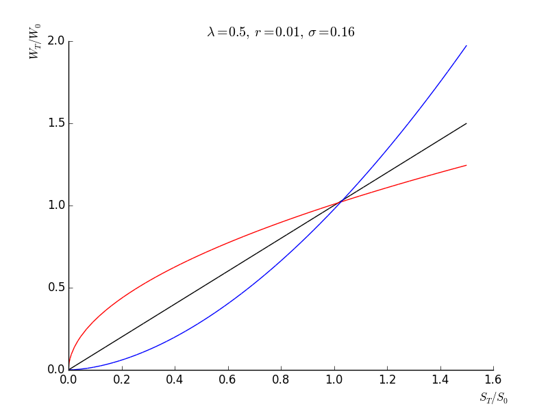
Relatively lengthy calculations also show that, setting: \[\alpha=\frac{\lambda}{\rho \sigma},\] we have: \[\frac{W_{T}^{*}}{W_{0}}=\exp\left((1-\alpha)(r+\frac{1}{2}\alpha\sigma^{2})T\right)R_{T}^{\alpha},\] where: \[R_{T}=\frac{S_{T}}{S_{0}}=\exp\left(rT+\sigma\lambda T+\sigma B_{T}\right).\]
Optimal wealth is thus a transformation of the stock return. The graph below gives the shape of this transformation for different values of parameters. For low risk aversion, the transformation is convex. It is concave for high risk aversion, and linear for \(\alpha=1\). This is consistent with the idea that investors with low risk aversion will accept the downside to benefit from the downside. In contrast, high risk aversion investors are willing to sacrifice the upside to protect the downside.
- The martingale method does not deliver a trading policy. We know from dynamic programming however that the optimal policy consists in investing \(\alpha\) on the stock at all times. Low risk aversion investors have \(\alpha>1\) (leverage) while high risk aversion investors have \(\alpha<1\) (the investor holds cash in addition to stocks). The case \(\alpha=1\) consists in putting all wealth on stocks and holding it subsequently. It is a buy-and-hold policy. It should be noted that in all cases, wealth is entirely consumed when \(R_{T}=0\). In contrast, an investor who splits its wealth on cash and stocks and never rebalances is guaranteed to keep its cash when the value of the stock goes to zero.