Static Portfolio Choice

October 7th, 2014

In this section of the course, I review the static portfolio choice problem. The investor chooses a portfolio structure which is then left alone. The investment criterion is the expected utility of wealth at a terminal date. I briefly review specifications for the utility function together with risk aversion concepts. I look at the case of constant absolute risk aversion and normal returns, with or without labour income. I then introduce mean variance preferences, linking them to expected utility. Mean variance with and without a risk free asset is studied. The link between mean variance preferences and the expected returns/beta relationship is explained (the key ingredient of the CAPM). I then touch on the implementation problem.

Timing

Two periods:
- portfolio decisions in t=0
- outcome observed in t=1
Outcomes in date \(1\) are uncertain as of date \(0\); they are described by random variables which we will identify in the notation using tildas
- \(x\): particular outcome; \(\tilde{x}\): random variable

Instruments

Instrument \(i\) with price \(p_{i}\) in period \(0\) gives right to pay-off \(\tilde{x}_{i}\) in period \(1\)
A cash instrument is an instrument with known date \(1\) pay-off as of date \(0\)
For risky assets, \(\tilde{x}\) is uncertain as of date \(0\)
I’ll assume there are \(N\) risky assets (\(i=1,\cdots,N\)) and potentially cash (the riskless asset), which will then have index \(0\)
The set of assets will be denoted by \(\cal{I}\), with either \({\cal I}=(1,\cdots,N)\) (no riskless asset) or \({\cal I}=(0,\cdots,N)\) (with a riskless asset)

Returns

The return of an instrument with price \(p\) and pay-off \(\tilde{x}\) is: \[\tilde{R}=\frac{\tilde{x}}{p}\]
The rate of return is \(\tilde{r}=\tilde{R}-1\)
The rate of return of cash is usually denoted \(r^{f}\); it is known as of date \(0\)

Investment and returns

From investment to pay-off
From \(t=0\) to \(t=1\):
- \(\phi \longrightarrow \tilde{R}\phi\)
- \(\phi \longrightarrow (1+\tilde{r})\phi\)

Portfolios

Wealth in period \(0\) is \(w_{0}\)
The portfolio is invested in period \(0\); quantities \((\theta_{i})_{i \in \cal{I}}\) are purchased
They need to satisfy: \[\sum_{i \in \cal{I}}\theta_{i}p_{i}=w_{0}\]
One can choose as control variables:
- quantities \((\theta_{i})_{i \in \cal{I}}\)
- dollar amounts invested on instruments \((\phi_{i})_{i \in \cal{I}}\) with \(\phi_{i}=\theta_{i}p_{i}\)
- wealth shares \((\pi_{i})_{i \in \cal{I}}\), with \(\pi_{i}=\phi_{i}/w_{0}\)

Budget constraints

Quantities: \[\sum_{i \in \cal{I}}\theta_{i}p_{i}=w_{0}\]
Dollar amounts: \[\sum_{i \in \cal{I}}\phi_{i}=w_{0}\]
Wealth shares: \[\sum_{i \in \cal{I}}\pi_{i}=1\]

Borrowing

Borrowing is best understood as a negative position in cash:
- from \(t=0\) to \(t=1\)
- \(\phi=-d \longrightarrow -d(1+r^{f})\)

Accounting for future wealth

for a given initial wealth \(w_{0}\), a portfolio allocation leads to a random final wealth \(\tilde{w}\) with:
- quantities: \(\tilde{w}=\sum_{i \in \cal{I}}\theta_{i}\tilde{x}_{i}\)
- invested amounts: \(\tilde{w}=\sum_{i \in \cal{I}}\phi_{i}\tilde{R}_{i}\)
- wealth shares: \(\tilde{w}=w_{0}\sum_{i \in \cal{I}}\pi_{i}\tilde{R}_{i}\)
- It is sometimes useful to introduce at date \(1\) an exogenous income (amount to be received) or liability (amount to be paid) \(\tilde{y}\)
- \(\tilde{w}=\tilde{y}+\sum_{i \in \cal{I}}\theta_{i}\tilde{x}_{i}\)
- \(\tilde{w}=\tilde{y}+\sum_{i \in \cal{I}}\phi_{i}\tilde{R}_{i}\)
- \(\tilde{w}=\tilde{y}+w_{0}\sum_{i \in \cal{I}}\pi_{i}\tilde{R}_{i}\)

Some return arithmetic

Without liability, we have:
- portfolio return: \[\tilde{R_{p}}=\frac{\tilde{w}}{w_{0}}=\sum_{i \in \cal{I}}\pi_{i}\tilde{R}_{i}\]
- portfolio rate of return: \[\tilde{r_{p}}=\frac{\tilde{w}}{w_{0}}=\sum_{i \in \cal{I}}\pi_{i}\tilde{r}_{i}\] (since \(\sum_{i \in \cal{I}}\pi_{i}=1\))

The space of excess returns

In the presence of a riskless asset, it is convenient to introduce excess returns versus the riskless rate: \[\tilde{r_{p}} = \sum_{i \in \cal{I}}\pi_{i}\tilde{r}_{i}\] \[=r^{f}+\sum_{i=1}^{N}\pi_{i}(\tilde{r}_{i}-r^{f}).\]
The choice variables are initially \((\pi_{i})_{i \in \cal{I}}\), under the constraint \(\sum_{i \in \cal{I}}\pi_{i}=1\).
In the excess return space, the choice variables are \((\pi_{i})_{i=1}^{N}\) to which no budget constraint applies since it is enforced by \(\pi_{0}=1-\sum_{i=1}^{N}\pi_{i}\).

The portfolio problem

Future wealth is a random variable, with a specific distribution
The portfolio problem:
- choose quantities (amounts, wealth shares) so as to obtain the best wealth distribution possible
How do we compare random outcomes?
- expected utility (Von Neumann Morgenstern - VNM) of outcome: \(E[u(\tilde{w})]\)
- the utility function embodies attitudes towards risk of the decision maker

Some remarks

The optimization problem cannot have a solution if there are arbitrage opportunities
Reminder: an arbitrage is a way to generate a strictly positive pay-off without committing any funds
The existence of a solution to a portfolio optimization problem thus guarantees the existence of a strictly positive stochastic discount factor (see below). We will see this principle in action

Arbitrage, the law of one price and SDFs

A stochastic discount factor is a random variable \(\tilde{m}\) such that for any pay-off \(\tilde{x}\), the market price can be recovered: \[p=E[\tilde{m}\tilde{x}].\]
The law of one price is equivalent to the existence of a stochastic discount factor. The absence of arbitrage is equivalent to the existence of an almost everywhere strictly positive discount factor. Broadly speaking, strict positivity ensures that a (possibly synthetic) asset with strictly positive payoff cannot have a strictly negative price (this would be an arbitrage).
In the return space, the above relationship reads: \[E[\tilde{m}\tilde{R}]=1.\]
The expectation of the discount factor is linked to the risk free rate: \[E[\tilde{m}](1+r^{f})=1.\]
In the excess return space, this reads: \[E[\tilde{m}(\tilde{r}-r^{f})]=0.\]
We thus have, in the presence of a risk free asset¹: \[E[\tilde{r}]-r^{f}=-R^{f}\text{cov}(\tilde{m},\tilde{R}),\] which describes the structure of risk premia across assets as a result of the covariances with the SDF.

Reminder on utility functions (1)

VNM utility functions are determined up to a linear transformation
Absolute risk aversion: \(\alpha(w)=-u''(w)/u'(w)\)
Relative risk aversion: \(\rho(w)=w\alpha(w)\)
Risk tolerance: \(\tau(w)=1/\alpha(w)\)
Additive certainty equivalent: for a centered distribution \(\tilde{\varepsilon}_{a}\) and an initial level of wealth \(w\), find \(\pi_{a}(w,\tilde{\varepsilon}_{a})\) such that: \[u(w-\pi_{a})=E[u(w+\tilde{\varepsilon}_{a})].\]
Multiplicative certainty equivalent: for a centered distribution \(\tilde{\varepsilon}_{m}\) and an initial level of wealth \(w\), find \(\pi_{m}(w,\tilde{\varepsilon}_{m})\) such that: \[u(w(1-\pi_{m}))=E[u(w(1+\tilde{\varepsilon}_{m}))].\]

Reminder on utility functions (2)

For small (centered) additive risks of variance \(\sigma^{2}\): \(\pi_{a} \approx \frac{1}{2}\sigma_{a}^{2}\alpha(w)\)
For small (centered) multiplicative risks of variance \(\sigma^{2}\): \(\pi_{m} \approx \frac{1}{2}\sigma_{m}^{2}\rho(w)\)

Some important utility functions

CARA: \(u(w)=-\exp(-\alpha w)\)
- range: \(\mathbb{R}\)
- absolute risk aversion: \(\alpha(w)=\alpha\)
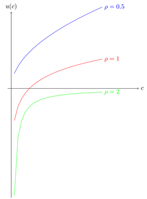
CRRA: \[u_{\rho}(w)= \frac{c^{1-\rho}}{1-\rho},\, \rho \geq 0,\, \rho\neq 1,\] \[u_{\rho}(w)=\log(w),\, \rho=1,\]
- range \(\mathbb{R}_{+}^{*}\)
- relative risk aversion: \(\rho(w)=\rho\)

CRRA utility functions - fig 1

Utility functions and return distributions

Utility functions often have a restricted domain (frequently: positive consumption)
Assumptions on return distributions have to be consistent
For example, CRRA models require \(\tilde{R}\geq 0\) i.e. \(\tilde{r} \geq -1\). This assumption is sometimes called ‘limited liability’: the owner of an asset cannot end up having to transfer cash to the issuer.
This is a problem mainly for discrete time models (or continuous times models where prices can jump)

Absolute or relative?

The key consideration is the dependence of risk attitudes vis-à-vis the level of wealth
- intuition suggests people accept greater dollar risk as their wealth rises

An important benchmark: CARA & normally distributed returns

Note that with normal returns, returns can be arbitrarily negative (no limited liability). Accordingly, the range of the utility function is \(\mathbb{R}\).
I assume that there is no labor income
\(\pmb{\pi}=(\pi_{i})_{i \in \cal{I}}'\) \[\underset{\pmb{\pi}}{\text{max}} \; E[-\exp(-\alpha \tilde{w})]\] \[\text{s.t.}:\] \[\tilde{w}=w_{0}\sum_{i \in \cal{I}}\pi_{i}\tilde{R}_{i}\] \[\sum_{i \in \cal{I}}\pi_{i}=1.\]

CARA normal case (1)

The random variable \(\tilde{w}\) is normally distributed. In this case, we know that: \[E[-\exp(-\alpha\tilde{w})] =\; -\exp(-\alpha E[\tilde{w}]+(\alpha^{2}/2)V[\tilde{w}])]\] \[=u(E[\tilde{w}]-(\alpha/2)V[\tilde{w}]).\]
Given that the function \(u(\cdot)\) is increasing, the program consists in maximizing the certainty equivalent \(E[\tilde{w}]-(\alpha/2)V[\tilde{w}]\), which reads, mean wealth minus the variance of wealth weighted by one half absolute risk aversion.

CARA normal case (2)

Preferences over the distribution of final wealth are thus entirely determined by the mean and the variance of the wealth distribution. This is an example of mean variance preferences.
We have: \[\tilde{w}=w_{0}\sum_{i \in \cal{I}}\pi_{i}\tilde{R}_{i}=w_{0}+w_{0}\sum_{i \in \cal{I}}\pi_{i}\tilde{r}_{i}\]
The maximized criterion is thus (dividing by \(w_{0}>0\)): \[E[\sum_{i \in \cal{I}}\pi_{i}\tilde{r}_{i}]-(\alpha w_{0}/2)V[\sum_{i \in \cal{I}}\pi_{i}\tilde{r}_{i}].\]

CARA normal case (3)

This is a standard mean-variance criterion, up to the fact that the risk aversion parameter depends on the level of wealth.
- if this was not the case, optimal portfolio composition would be independent of the wealth level; this would imply that the investor take more dollar risk at higher wealth levels; in the CARA case, the appetite for dollar risk is independent of the level of wealth; thus the correction.

When do we get mean variance preferences?

How general is mean variance ?
- preferences induced by utility functions will not, in general, correspond to mean-variance; additional assumptions are needed.
- when the distribution of portfolio returns is characterized by mean and variance, all utility functions naturally lead to mean variance preferences (see elliptic distributions).
- in the presence of stochastic labour income, mean variance needs to be amended

CARA normal case (4)

In the presence of normally distributed stochastic labor income, the optimal programme is: \[\underset{\pmb{\pi}}{\text{max}} \; E[-\exp(-\alpha \tilde{w})]\] \[\text{s.t.}\] \[\tilde{w}=\tilde{y}+\sum_{i \in \cal{I}}\theta_{i}\tilde{x}_{i}\] \[\sum_{i \in \cal{I}}\theta_{i}p_{i}=w_{0}.\]
It is this time more convenient to take as control variables the quantities: \((\theta_{i})_{i \in {\cal I}}\).

CARA normal case (5)

As before, we need to maximize the certainty equivalent: \(E[\tilde{w}]-(\alpha/2)V[\tilde{w}]\). This is equivalent to maximizing: \[E\left[\sum_{i \in {\cal I}}\theta_{i}\tilde{x}_{i}\right]-(\alpha/2)V\left[\tilde{y}+\sum_{i \in {\cal I}}\theta_{i}\tilde{x}_{i}\right].\]
We can decompose the variance term as: \[V\left[\tilde{y}\right]+V\left[\sum_{i \in \cal{I}}\theta_{i}\tilde{x}_{i}\right] +2\text{Cov}\left(\sum_{i \in \cal{I}}\theta_{i}\tilde{x}_{i},\tilde{y}\right).\]

CARA normal case (6)

I give the result assuming there is a riskless asset.
We assume the price of cash is \(p_{0}=1\), and the payoff \(\tilde{x}_{0}=1+r^{f}\).
Using the budget constraint \(\theta_{0}=w_{0}-\sum_{i=1}^{N}\theta_{i}p_{i}\), we can rewrite the criterion as: \[E\left[w_{0}(1+r^{f})+\sum_{i=1}^{N}\theta_{i}(\tilde{x}_{i}-p_{i}(1+r^{f}))\right]-(\alpha/2)V\left[\tilde{y}+\sum_{i=1}^{N}\theta_{i}\tilde{x}_{i}\right].\]
Notation:
- \(\theta\) is the \(N\times 1\) vector of quantities invested on each risky asset
- \(V[\tilde{x}]\) is the \(N\times N\) matrix where each \((i,j)\) is the covariance of the pay-offs of asset \(i\) and \(j\). It is assumed to have full rank, so that no financial asset is riskless or redundant.
- \(\text{Cov}(\tilde{x},\tilde{y})\) is the \(N\times 1\) vector where each entry measures the covariance of a financial instrument with labour income
- \(E[\tilde{\tilde{x}}]\) is the \(N\times 1\) vector of the expected excess pay-offs \((\tilde{x}_{i}-p_{i}(1+r^{f}))\) of the risky instruments instruments.

CARA normal case (7)

The first order condition leads to, in matrix notation: \[\theta=V[\tilde{x}]^{-1}\left(-\text{Cov}(\tilde{x},\tilde{y})+\frac{1}{\alpha}E[\tilde{\tilde{x}}]\right).\]
Remember that \(1/\alpha\) is risk tolerance.
The structure of the solution is as follows: the optimal porfolio consists of a hedging portfolio (which tries to replicate income variability using financial assets) and a speculative portfolio which has the same structure as in the case without labour income. The latter portfolio receives a weight equal to risk tolerance.

Optimization and SDF

I assume there is a solution \(\pmb{\pi}_{*}\) to the following problem: \[\underset{\pmb{\pi}}{\text{max}} \; E[u(\pmb{\pi}'\pmb{\tilde{R}})]\] \[\text{s.t.}\] \[\pmb{\pi}'\pmb{e}=1,\] where \(\pmb{e}\) is a vector where all components are equal to \(1\), and \(\pmb{\pi}\) is the vector of asset proportions.
The Lagrangian reads: \[{\cal L}=E[u(\pmb{\pi}'\pmb{\tilde{R}})]-\gamma \pmb{\pi}'\pmb{e},\] and the first order condition reads: \[E[u'(\pmb{\pi}'\pmb{\tilde{R}})\pmb{\tilde{R}}]=\gamma \pmb{e}.\]
Let: \[\tilde{m}=\frac{u'(\pmb{\pi}_{*}'\pmb{\tilde{R}})}{\gamma}.\] We then have: \[E[\tilde{m}\pmb{\tilde{R}}]=\pmb{e},\] i.e. for any asset \(i\): \[E[\tilde{m}\tilde{R}_{i}]=1.\] In other words, we have built an SDF from the solution of the optimization problem.

Mean variance efficiency

A portfolio \(p\) with mean and variance \((\mu_{p},\sigma_{p})\) is dominated by a portfolio \(q\) with mean and variance \((\mu_{q},\sigma_{q})\) if \(\mu_{q} \ge \mu_{p}\) and \(\sigma_{q} \le \sigma_{p}\) with at least one inequality being strict.
A portfolio is efficient in the mean variance sense if it is not dominated by any other portfolio.
Domination is a preorder. An efficient portfolio is a maximal element for the preorder. In particular, it is not a total order (all portfolio pairs cannot necessarily be ordered).

Mean variance without a riskfree asset (1)

The program: it consists in minimizing portfolio variance for a given level of expected returns \[\underset{\pmb{\pi}}{\text{min}} \; V\left[\sum_{i=1}^{N}\pi_{i}\tilde{r}_{i}\right]=\pmb{\pi}' \Sigma \pmb{\pi}\] \[\text{s.t.}\] \[\sum_{i=1}^{N}\pi_{i}=\pmb{\pi}'\pmb{e}=1\] \[E\left[\sum_{i=1}^{N}\pi_{i}\tilde{r}_{i}\right]=\pmb{\pi}'\pmb{\mu}=\mu_{p}.\]

Mean variance without a riskfree asset (2)

Bold notations denote vectors
- \(\Sigma\) is the covariance matrix of returns, which we assume invertible
- \(\pmb{e}\) is a vector of ones
- \(\pmb{\tilde{r}}\) is the vector of returns
- \(\pmb{\mu}\) is the vector of expected returns
We assume \(\pmb{\mu}\neq \pmb{e}\) to avoid degeneracy

Mean variance without a riskfree asset (3)

Lagrangian for the optimization problem (a factor \(1/2\) is convenient): \[\frac{1}{2}\pmb{\pi}' \Sigma \pmb{\pi}-\delta (\pmb{\pi}'\pmb{\mu}-\mu_{p})-\gamma (\pmb{\pi}'\pmb{e}-1)\] where I have introduced the Lagrange multipliers \(\delta\) and \(\gamma\).
The necessary and sufficient first order condition (positive definite quadratic problem) is: \[\Sigma \pmb{\pi}=\delta \pmb{\mu}+\gamma \pmb{e},\] or, assuming the covariance matrix is invertible: \[\pmb{\pi}=\delta\Sigma^{-1}\pmb{\mu}+\gamma \Sigma^{-1}\pmb{e}.\]

Mean variance without a riskfree asset (4)

Injecting this into the constraints leads to a system for the Lagrange multipliers: \[\delta \pmb{\mu}' \Sigma^{-1}\pmb{\mu}+\gamma \pmb{\mu}' \Sigma^{-1}\pmb{e}=\mu_{p},\] \[\delta \pmb{e}'\Sigma^{-1}\pmb{\mu}+\gamma \pmb{e}'\Sigma^{-1}\pmb{e}=1.\]
Reminder: \[\begin{pmatrix} a&b\\ c&d \end{pmatrix}^{-1}=\frac{1}{ad-bc}\begin{pmatrix} d&-b\\ -c&a \end{pmatrix}\]
It is useful to introduce two specific portfolios: \[\pmb{\pi}_{1}=\frac{1}{\pmb{e}'\Sigma^{-1}\pmb{e}}\Sigma^{-1}\pmb{e},\] \[\pmb{\pi}_{\mu}=\frac{1}{\pmb{e}'\Sigma^{-1}\pmb{\mu}}\Sigma^{-1}\pmb{\mu}.\]

Mean variance without a riskfree asset (5)

We can write : \[\pmb{\pi} = (\delta\pmb{e}'\Sigma^{-1}\pmb{\mu})\pmb{\pi}_{\mu}+(\gamma\pmb{e}'\Sigma^{-1}\pmb{e})\pmb{\pi}_{1}=\] \[\lambda \pmb{\pi}_{\mu}+(1-\lambda) \pmb{\pi}_{1}.\]
Thus, any optimal portfolio is a combination of the two portfolios we singled out:
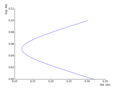
- \(\pmb{\pi}_{1}\) is the minimum variance portfolio
- \(\pmb{\pi}_{\mu}\) is another portfolio as soon as \(\pmb{\mu} \neq \pmb{e}\)

Mean variance without a riskfree asset (6)

\(A=\pmb{\mu}'\Sigma^{-1}\pmb{\mu}\), \(B=\pmb{\mu}'\Sigma^{-1}\pmb{e}\), \(C=\pmb{e}'\Sigma^{-1}\pmb{e}\). \[\lambda=\frac{BC\mu_{p}-B^{2}}{AC-B^{2}},\] \[\sigma_{p}^{2}=\frac{A-2B\mu_{p}+C\mu_{p}^{2}}{AC-B^2{}}.\]
Check this.
The efficient frontier (in the standard deviation mean space) is the subset of non dominated portfolios in the set: \[\{(\sigma_{p},\mu_{p}),\; \mu_{p}\geq \mu_{1}\}\] where \(\mu_{1}=\pmb{\pi}_{1}'\pmb{\mu}\).

Mean variance without a riskfree asset (7) - fig 2

Figure 2: Efficient Frontier (without a risk free asset)

Mean variance without a riskfree asset (8)

I list the technical conditions below:
- we assume that \(\pmb{\mu}\) and \(\pmb{e}\) are not colinear
- we assume \(\pmb{e}'\Sigma^{-1}\pmb{\mu>0}\)
- we have \(\pmb{e}'\Sigma^{-1}\pmb{e}>0\) as \(\Sigma^{-1}\) defines a positive definite quadratic form
- we have \(\left(\pmb{\mu}'\Sigma^{-1}\pmb{e}\right)^2<\left(\pmb{e}'\Sigma^{-1}\pmb{e}\right)\left(\pmb{\mu}'\Sigma^{-1}\pmb{\mu}\right)\) from the Cauchy-Schwartz inequality and \(\pmb{e}'\Sigma^{-1}\pmb{e}>0\).

Mean variance with a riskfree asset (1)

It is convenient in this case to use the notation \(\pmb{\pi}\) to denote the vector of positions on the risky assets (see the slide on the space of excess returns). The cash position is thus: \[\pi_{0}=1-\pmb{e}'\pmb{\pi}.\]
The vector \(\pmb{\pi}\) is unconstrained. The optimization problem can be written: \[\underset{\pmb{\pi}}{\text{min}} \; \pmb{\pi}' \Sigma \pmb{\pi}\] \[\text{s.t.}\] \[\pmb{\pi}'(\pmb{\mu}-r^{f}\pmb{e})=\mu_{p}-r^{f}.\]
For reasons that will be clear below, I assume \(\pmb{e}'\Sigma^{-1}(\pmb{\mu}-r^{f}\pmb{e})>0\).

Mean variance with a riskfree asset (2)

First order condition for the Lagrangian: \(\pmb{\pi}=\delta \Sigma^{-1}(\pmb{\mu}-r^{f}\pmb{e})\)
From \((\pmb{\mu}-r^{f}\pmb{e})'\pmb{\pi}=\mu_{p}-r^{f}\), we get the value of \(\delta\) and then the value of \(\pmb{\pi}\): \[\pmb{\pi}=\frac{\mu_{p}-r^{f}}{(\pmb{\mu}-r^{f}\pmb{e})'\Sigma^{-1}(\pmb{\mu}-r^{f}\pmb{e})}\Sigma^{-1}(\pmb{\mu}-r^{f}\pmb{e}).\]
The standard deviation of the portfolio is: \[\frac{|\mu_{p}-r^{f}|}{\sqrt{(\pmb{\mu}-r^{f}\pmb{e})'\Sigma^{-1}(\pmb{\mu}-r^{f}\pmb{e})}}.\]

Mean variance with a riskfree asset (3)

The tangency portfolio is: \[\pmb{\pi_{*}}=\frac{1}{\pmb{e}'\Sigma^{-1}(\pmb{\mu}-r^{f}\pmb{e})}\Sigma^{-1}(\pmb{\mu}-r^{f}\pmb{e}).\]
It is a portfolio fully invested in risky assets which is on the overall efficient frontier. It is thus also on the risky asset efficient frontier.

Mean variance with a riskfree asset (4) - fig 3

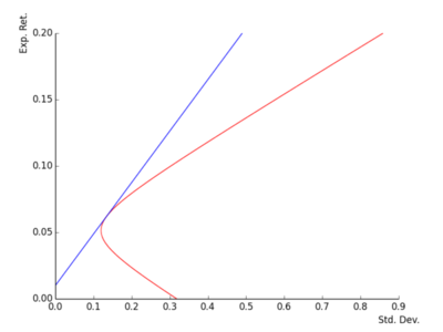
Figure 3: Efficient Frontier (with risk free asset)

Mean variance with a riskfree asset (4) - fig4

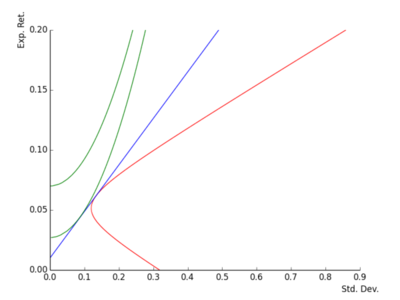
Figure 4: Efficient Frontier (with risk free asset): iso-utility curves

Data for the graphs (1)

Two risky assets:
- \(\mu_{1}=0.05,\, \sigma_{1}=0.12\)
- \(\mu_{2}=0.07,\, \sigma_{2}=0.16\)
- \(\rho=0.7\)
- \((\mu_{1}-r)/\sigma_{1}=0.33\)
- \((\mu_{2}-r)/\sigma_{2}=0.375\)
- \(\pmb{\pi_{1}}=(0.93,0.07)\)
- \(\text{vol}(\pmb{\pi_{1}})=0.12\)
- \(\pmb{\pi_{*}}=(0.4,0.6)\)
- \(\text{vol}(\pmb{\pi_{*}})=0.13\)
- \(\text{sharpe}(\pmb{\pi_{*}})=0.39\)

Data for the graphs (2)

The graphs shown assume positive Sharpe ratios for the underlying assets. This is the ‘normal’ situation. It ensures that the efficient frontier (with a riskfree asset!) is upward sloping.

A different description of the efficient frontier (1)

Maximize the expected return penalized for portfolio variance (\(\rho>0\)): \[\underset{\pmb{\pi}}{\text{max}} \; r^{f}+\pmb{\pi}'(\pmb{\mu}-r^{f}\pmb{e})-\frac{\rho}{2}\pmb{\pi}' \Sigma \pmb{\pi}.\]
Exercise: recover the lagrange multiplier of the traditional approach
The criteria are given by quadratic utility functions, indexed by \(\rho\)

A different description of the efficient frontier (2)

The first order condition reads: \[(\pmb{\mu}-r^{f}\pmb{e})=\rho\Sigma \pmb{\pi},\] and this implies that the optimal portfolio is proportional to the tangency portfolio.
How much of the tangency portfolio \(\pmb{\pi_{*}}\) does an investor with the above preferences and beliefs buy?
From the first order condition of the utility maximization problem², we get that the weight \(\hat{\pi}=1-\pi_{0}\) invested in the tangency portfolio is: \[\hat{\pi}=\frac{1}{\rho}\frac{\mu_{*}-r^{f}}{\text{var}(\tilde{r}_{*})}.\]
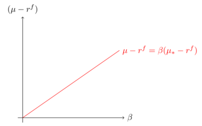
We will remember that: \[\rho \hat{\pi}=\frac{\mu_{*}-r^{f}}{\text{var}(\tilde{r}_{*})},\] which is therefore independent of the risk aversion level of the investor. This will play a role in the derivation of the CAPM.

Interpretation of the first order condition (1)

Consider that the optimal portfolio of a mean-variance investor (\(p\) with weights \(\pmb{\pi}\)) is tilted by adding a long-short portfolio \(\pmb{\pi}_{\delta}\). How does that affect quadratic utility?
The utility level changes by (first order approximation): \[\mu_{\delta}-\rho\text{cov}(\tilde{r}_{\delta},\tilde{r}_{p})\] \[=\mu_{\delta}-\rho\frac{\text{cov}(\tilde{r}_{\delta},\tilde{r}_{p})}{\text{var}(\tilde{r}_{p})}\text{var}(\tilde{r}_{p}),\] \[=\mu_{\delta}-\rho \beta (\tilde{r}_{\delta},\tilde{r}_{p}) \text{var}(\tilde{r}_{p}),\] \[=\mu_{\delta}-\rho \hat{\pi}\beta (\tilde{r}_{\delta},\tilde{r}_{*}) \text{var}(\tilde{r}_{*}).\]

Interpretation of the first order condition (2)

Because the quantity \(\rho \hat{\pi}\) is independent of \(\rho\), the trade off between return and beta is a well defined consequence of the mean and variance assumptions.
Injecting the value of \(\rho \hat{\pi}\) into the first order condition delivers the quantity: \[\mu_{\delta}-(\mu_{*}-r^{f})\beta (\tilde{r}_{\delta},\tilde{r}_{*}).\]
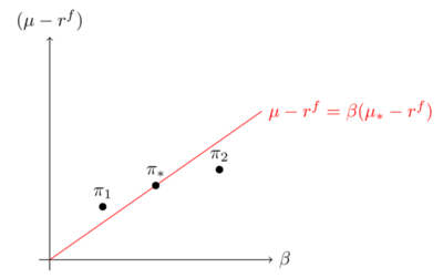
Given the optimality of the tangency portfolio, the above quantity should be zero for all long short deviations to the tangency portfolio: \[\mu_{\delta}=(\mu_{*}-r^{f})\beta (\tilde{r}_{\delta},\tilde{r}_{*}).\]
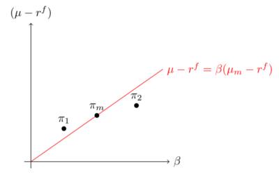
For long short portfolios which borrow to buy a stock, the condition reads: \[(\mu_{i}-r^{f})=(\mu_{*}-r^{f})\beta (\tilde{r}_{i},\tilde{r}_{*}).\]

Interpretation of the first order condition (3)

The above relationship embodies the return beta trade off embedded in the mean variance assumptions.
At this stage, no equilibrium assumption has been made. We are looking at the implications of a portfolio being mean-variance optimal.
Note that the tangency portfolio can be replaced by any other efficient portfolio in the relationship.

The excess return-beta relationship (1) - fig 5

The excess return-beta relationship (2) - fig 6

The two fund theorem and the CAPM

We now move to equilibrium considerations. We assume all investors share the same beliefs on expected returns and risk, and all choose mean variance efficient portfolios.
As a result, they all hold a mixture of the risk free asset and a unique portfolio of risky asset, the tangency portfolio.
This is an instance of the two fund theorem, which also holds in more general contexts
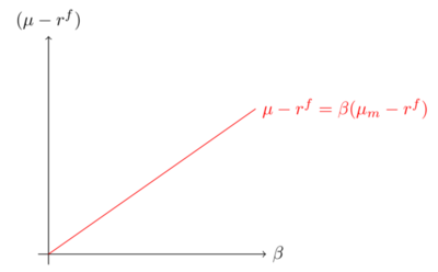
The risky asset portfolio should be equal to the market portfolio of risky asset, with return \(r_{m}\). This gives: \[(\mu_{i}-r^{f})=(\mu_{m}-r^{f})\beta (\tilde{r}_{i},\tilde{r}_{m}).\]

Illustration of the CAPM - fig 7

The low beta anomaly - fig 8

Equity pricing anomalies

Take an investment universe (stocks) and an equity index
Follow the steps:
- build equity portfolios by sorting stocks according to a financial characteristic
- compute the beta of the portfolios and graph realized returns against betas
- is the pricing error significant?
Examples of characteristics: size, book value, momentum, beta, vol
This procedure asks whether the index is mean variance efficient in sample
The pricing errors should be statistically significant

Mean variance in practice: the challenges

First, there is a question of interpretation: what is the investment horizon?
- in particular, this conditions the nature of the risky asset (bonds or cash).
One also needs to be clear on whether real returns or nominal returns are considered
Once this has been clarified, input data needs to be estimated:
- getting hold of expected returns
- getting hold of the covariance matrix
The optimal portfolio is very sensitive to inputs
- garbage in, garbage out

Examples of implementations

Give the same return to all risky assets
- this delivers the minimum variance portfolio, which is not optimal unless the expected returns are truly equal across assets
Link the return assumptions to the risk estimates
- this leads to various solutions…
For returns: estimate the payoffs of the asset and derive the implies return from the current asset price
Example: ERC ?